
Personal Research on Nonlinear Least Squares
Dates: Feb. 2021 - Sept. 2021
Context
When I learned about linear least squares and their closed form solution, during my first year in engineering school, I was already familiar with deep learning, so I noticed the similarity with the Mean Squared Error (MSE) loss. I wondered if there was a way to solve the optimization problem in a similar way.
Indeed, a single layer neural network with one output, an activation function $f$ and MSE loss, is equivalent to a linear least squares problem, which can be formulated as:
\[\arg\min_ {\theta\in\mathbb{R}^d}\mathcal{L}(\theta), \quad \mathcal{L}(\theta)= \sum_{i=1}^n \left( f(x_i^T \theta) - y_i \right)^2\]where $x_i\in\mathbb{R}^d$ are the inputs vectors, $y_i\in\mathbb{R}$ are the target outputs, and $\theta\in\mathbb{R}^d$ is the parameter to be estimated.
My algorithms
I tried to develop algorithms by myself (without looking at the literature) to solve this problem, and I ended up with a variant of the Iteratively Reweighted Least Squares (IRLS) algorithm.
The idea is to consider an alternative problem:
\[\arg\min_ {\theta\in\mathbb{R}^d}\mathcal{L}'(\theta), \quad \mathcal{L}'(\theta)=\frac{1}{2} \sum_{i=1}^n w_i \left( x_i^T \theta - z_i \right)^2\]with $z_i=f^{-1}(y_i)$ if $f$ is invertible. This has the closed form solution: $\theta = (X^T W X)^{-1} X^T W z$, where $W$ is a diagonal matrix with $w_i$ on the diagonal.
When computing the gradient of the two losses with respect to $\theta$, we can show that if we choose $w_i=f’(x_i^T\theta)\frac{f(x_i^T\theta) - y_i}{x_i^T\theta - z_i}$, then they are equal. This means that if we iteratively update $w_i$ and $\theta$ using the closed form solution, if the algorithm converges to $\theta^*$ (with $\nabla_\theta\mathcal{L’}(\theta^*)=0$), then $\nabla_\theta\mathcal{L}(\theta^*)=0$ (i.e. it is a local minima or maxima of the true loss)!
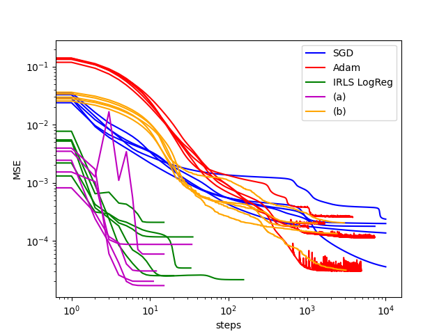
This algorithm ((a) in the figure below) has a few issues:
- $X^T W X$ may not be invertible. But as it is semidefinite positive, we can be sure that $X^T W X+\lambda I_d$ is invertible, for any $\lambda > 0$.
- the algorithm may never converge
- it may converge to a maxima
- matrix inversion is slow: I tried several variations to speed up the algorithm, without much success. The best one is (b) in the figure below.
I did not compare my algorithms with the literature, but I compared them with SGD and Adam. More recently, I noticed that my algorithm is also very similar to IRLS for logistic regression, so I included it in the benchmarks although logistic regression minimizes the negative log-likelihood instead of the MSE.
| Algorithm | Steps until convergence | Total time |
|---|---|---|
| SGD | 9453.8 | 250 ms |
| Adam | 3724.2 | 140 ms |
| IRLS LogReg | 51.6 | 44 ms |
| (a) | 17.4 | 15 ms |
| (b) | 2126.0 | 130 ms |
The results are quite good, however my algorithm doesn’t work as well with real data (I tried with the MNIST database). I think it is because the loss landscape is more complex, and the algorithm is not guaranteed to behave nicely.
As this work was done during my first year in engineering school, I did not have all the knowledge I have now, so I am sure that there are many things that could be improved. Still, it made me very familiar with the mathematical properties of linear least squares, and I learned a lot about optimization algorithms. I was able to easily get the highest grade for the “Statistics: linear models” course I took in second year!